重读AlexNet

https://proceedings.neurips.cc/paper_files/paper/2012/file/c399862d3b9d6b76c8436e924a68c45b-Paper.pdf

proceedings.neurips.cc/paper_files/paper/2012/file/c399862d3b9d6b76c8436e924a68c45b-Paper.pdf

Intro

After 12 years, reading Alexnet again can still give us insights.

This work comes from UoT, Alex Krizhevsky is first author, his others famous paper:

• https://scholar.google.com/citations?view_op=view_citation&hl=en&user=xegzhJcAAAAJ&citation_for_view=xegzhJcAAAAJ:9yKSN-GCB0IC
• https://scholar.google.com/citations?view_op=view_citation&hl=en&user=xegzhJcAAAAJ&citation_for_view=xegzhJcAAAAJ:d1gkVwhDpl0C
• https://scholar.google.com/citations?view_op=view_citation&hl=en&user=xegzhJcAAAAJ&citation_for_view=xegzhJcAAAAJ:u-x6o8ySG0sC

Abstract Part

Abstract part doesn’t really explain the network or any algorithms, but it points out AlexNet (In paper called ‘our network’) is much more better than the rank2 method in ImageNet competition, and it is a network with numerous params and trained on 2 GPUs, which are novel at 2012.

Conclusion Part

AlextNet paper doesnt have a namely ‘Conclusion’, instead it has a ‘Discussion’. These discussions are really smart even seen at today:

• Our results show that a large, deep convolutional neural network is capable of achieving recordbreaking results on a highly challenging dataset using purely supervised learning.

This start a new subject called ‘Deep Learning’. And finally we got ‘Scaling Law’ which bring us LLMs.

It is notable that our network’s performance degrades if a single convolutional layer is removed. For example, removing any of the middle layers results in a loss of about 2% for the top-1 performance of the network. So the depth really is important for achieving our results.

But this part is a little bit not making sense, cuz you compare different network’s depth but didnt control their params, some how you can still reach better results if you have larger ‘width’ but smaller ‘depth’.

To simplify our experiments, we did not use any unsupervised pre-training even though we expect that it will help, especially if we obtain enough computational power to significantly increase the size of the network without obtaining a corresponding increase in the amount of labeled data.

As we know scaling law now, this is not really true, after the model become much more larger, without significant amount of data, you will finally reach threshold.

What’s more. after 12 years we finally find it is really hard to get large amount of high quality labeled data, so unsupervised learning is relatively more important in current machine learning area.

Architecture Part

Architecture part first point out three novelty of this work:

• ReLU Nonlinearity
• Train on multiple GPUs
• Local Response Normalization
• Overlapping Pooling

ReLU

At that point, the main track of nn uses tanh and sigmoid. Alex use ReLU which is proposed from Abien Fred M. Agarap

sigmoid: $f(x) = 1 / {1 - e^{-x}}$ In deep networks, the gradients of the sigmoid function can become very small, especially for neurons in the early layers.

tanh: $f(x) = \frac{e^x - e^{-x}} {e^x + e^{-x}}$. The gradients are larger compared to the sigmoid function, which can help with the learning process.

Rectified Linear Units(ReLU): $f(x) = max(0, x)$. ReLU does not suffer from the vanishing gradient problem. Gradients are preserved better during backpropagation, which helps in training deep networks. ReLU introduces sparsity in the network by outputting zero for negative input values, which can lead to more efficient and faster computations. Also it is really easy to differentiate.

Train on multiple GPUs

Nowadays we call it “Distributed Training”, torch.distributed give us more efficient tools nowadays.

Local Response Normalization

This part AlexNet design a complex function to do normalization, seems he want to add spatial messages to normalization, but now we know it is not very important to do normalization, but it is important to design a good network. And we have relatively better normalization nowadays like epoch normalization and layer normalization.

Overlapping Pooling

This part this a tick, that AlexNet have overlapped pooling layers.

Overall Architecture

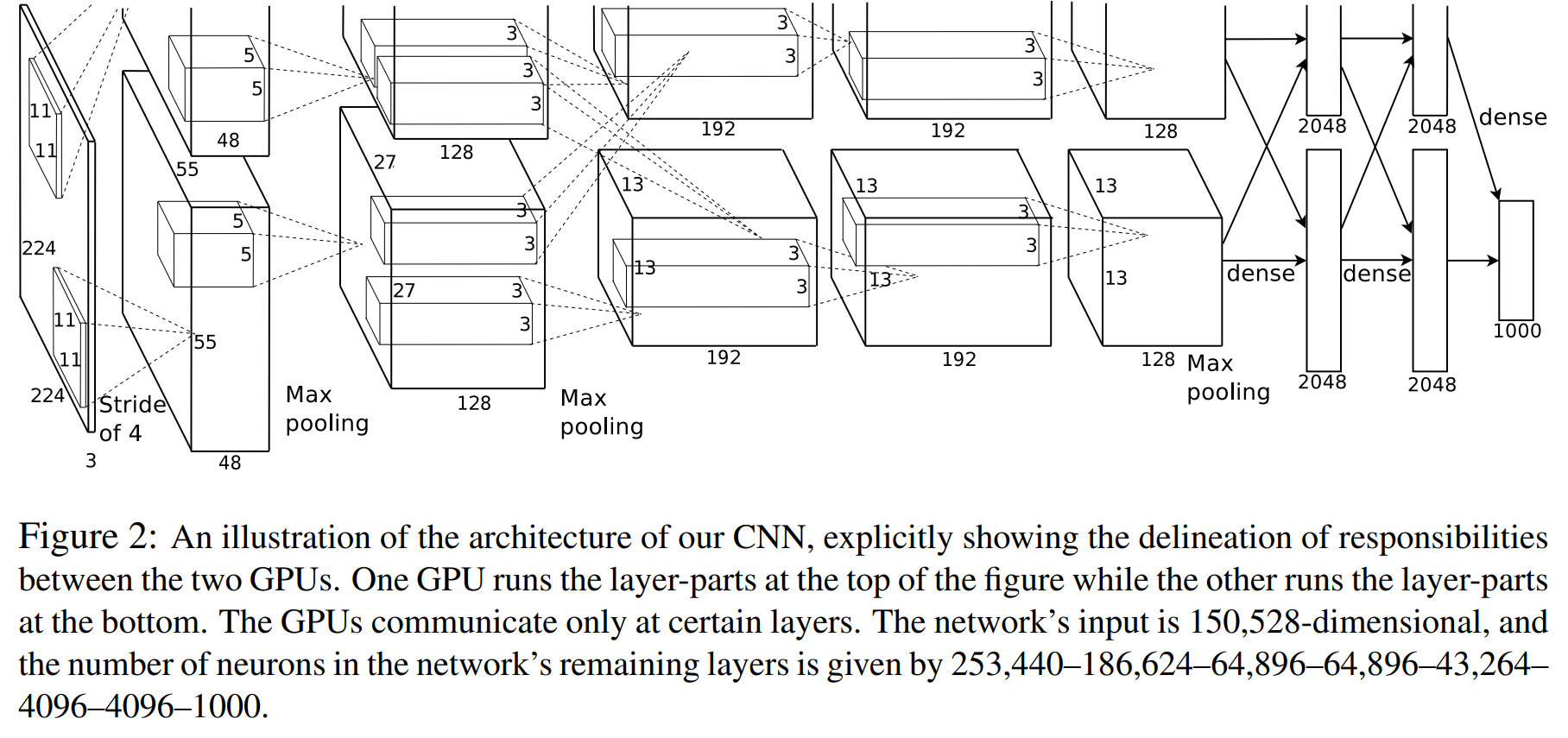
AlexNet is a type of CNN.

• The first convolutional layer filters the 224×224×3 input image with 96 kernels of size 11×11×3
  with a stride of 4 pixels. (And with 2 padding)

$\text { Output Size }=\left\lfloor\frac{(\text { Input Size }- \text { Filter Size }+2 \times \text { Padding })}{\text { Stride }}\right\rfloor+1$

So it will be:

$\text { Output Size }=\left\lfloor\frac{(\text { 224 }- \text { 11 }+2 \times \text { 2 })}{\text { 4 }}\right\rfloor+1 = \lfloor \frac{217}{4} \rfloor +1 = 54+1 = 55$

For the depth, it has two separate image so the depth is $\frac{96}{2} = {48}$

So we have:

• The second convolutional layer takes as input the (response-normalized and pooled) output of the first convolutional layer and filters it with 256 kernels of size 5 × 5 × 48.

Also need to mark:

• The third convolutional layer has 384 kernels of size 3 × 3 ×
  256 connected to the (normalized, pooled) outputs of the second convolutional layer.

Here AlexNet make the convolution results of second layer to both third layer, that means “The GPUs communicate only at certain layers.”

• The fully-connected layers have 4096 neurons each.

Data Part

Data Augmentation

• The first form of data augmentation consists of generating image translations and horizontal reflections. We do this by extracting random 224 × 224 patches (and their horizontal reflections) from the 256×256 images and training our network on these extracted patches

This doest really make sense cuz the new image are almost the same.

• The second form of data augmentation consists of altering the intensities of the RGB channels in
  training images.

But in fact at the dataset part AlexNet write “So we trained our network on the (centered) raw RGB values of the pixels.” So perhaps this hasnt use.

Dropout

At that time scientists think with drop out we can get several different models. but now we know it is same to L2 norm.

Dropout: A Simple Way to Prevent Neural Networks from Overfitting. By Nitish Srivastava, Geoffrey Hinton, Alex Krizhevsky, Ilya Sutskever, and Ruslan Salakhutdinov. UoT.

Results

The results are unprecedented good. But what is really worth thinking is the 6.1 Quotative Evaluation part.

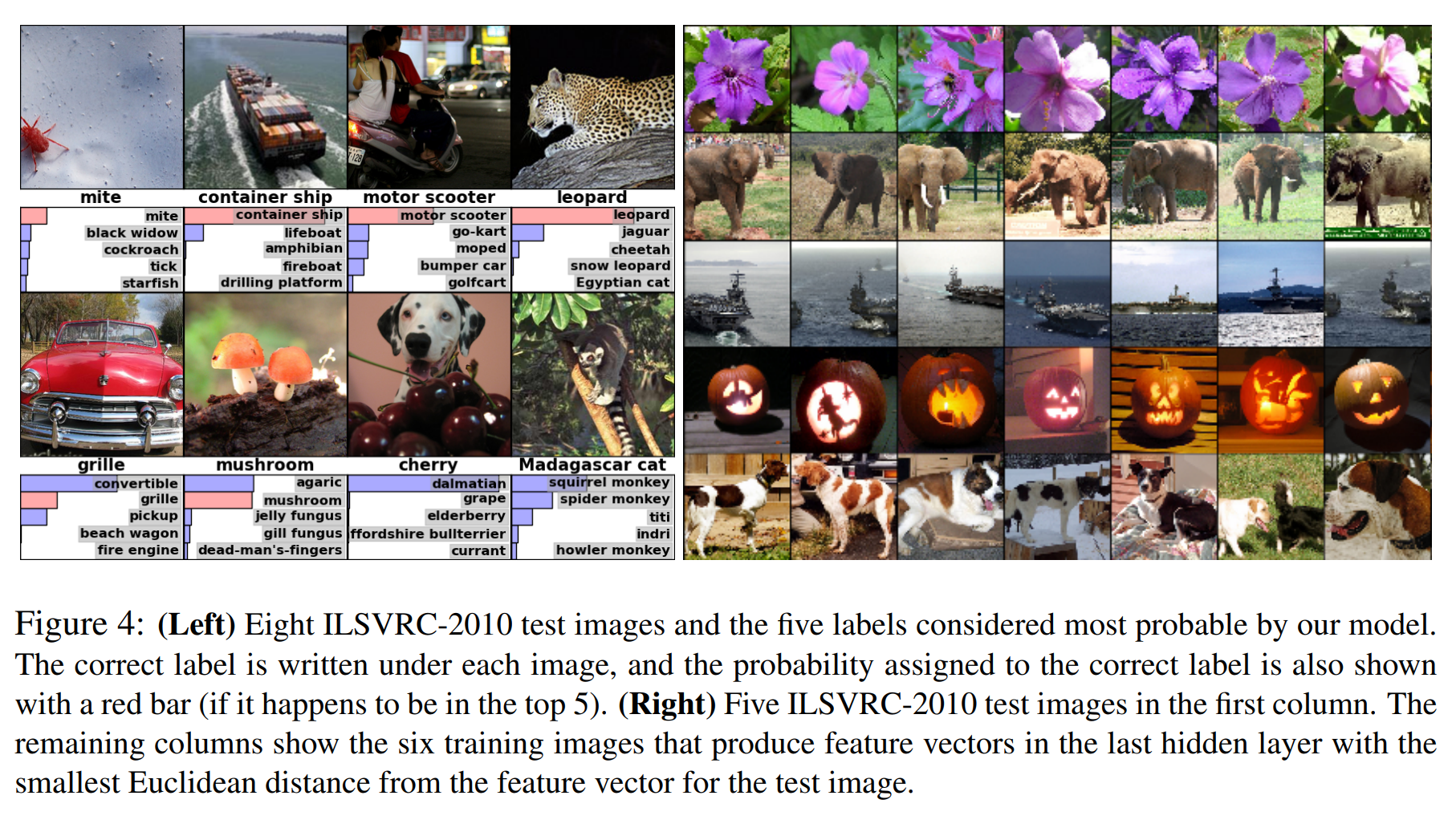
• Five ILSVRC-2010 test images in the first column. The remaining columns show the six training images that produce feature vectors in the last hidden layer with the smallest Euclidean distance from the feature vector for the test image.

This shows that CNN is really good at image embedding.