Mathematical Models and Life Choices

It has become a traditional behavior that when leaving Alibaba, employees will send a long post in the Alibaba blog. Here, I have prepared four short stories as a parting gift for Baba as I decided to leave industry and pursue my career in academia.

There are many interesting mathematical models in the world that can, to some extent, offer us a lot of insights.

Chinese Version: https://zhuanlan.zhihu.com/p/871793375

Career Journey

Keywords: Markov Decision Process

Students who have studied probability theory are likely familiar with the Markov process. In the field of reinforcement learning, this theory is extended to the Markov Decision Process (MDP), where an Agent’s behavior optimization within this process is fascinating and offers valuable insights for our career paths.

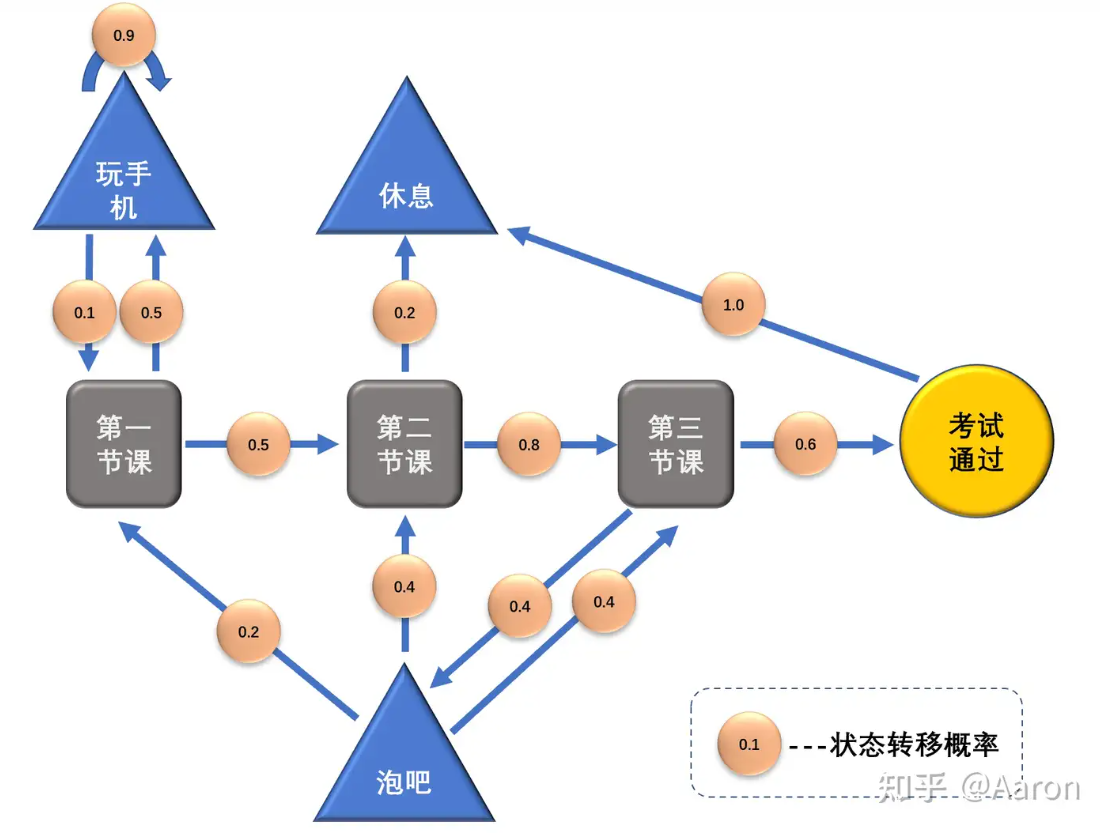
In a classic Markov process, state transitions are random. For example, a student might currently be in a lecture with a 50% chance of transitioning to a “playing on phone” state and a 50% chance of going to the next lecture, represented as follows:

We can extend this process: the Agent can earn certain rewards throughout the process. Attending lectures has a negative reward (since it’s challenging), while hanging out at the bar has a positive reward (since it’s enjoyable), as illustrated below:

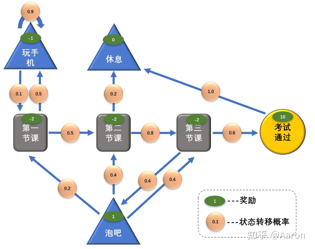
Markov Decision Theory aims to calculate the optimal strategy for the Agent. If one only focuses on the reward of hanging out (+1), they might avoid attending lectures with a reward of -2 and eventually fail to achieve a higher reward like passing exams (+10).

The MDP is defined as follows:

MDP = (S, A, P, R, γ)

Where:

• State Space (S): The set of all possible states, covering lecture attendance, hanging out, passing exams, etc.
• Action Space (A): The set of actions available in each state.
• Transition Probability §: The state transition function.
• Reward Function ®: The immediate reward obtained after transitioning to another state.
• Discount Factor (\( \gamma \)): Used to discount future rewards, reflecting the degree of emphasis on long-term gains.

For a specific MDP, an Agent can have a policy \( \pi \), representing the probability of choosing action \( a \) in state \( s \):

\[ \pi(a | s) = P[A_t = a | S_t = s] \]

A policy fully defines an individual’s behavior, specifying all possible actions in various states along with their probabilities.

Given a particular policy \( \pi \), the value of the policy can be calculated using the Bellman equation. The value of each state is:

The value for each state-action pair is:

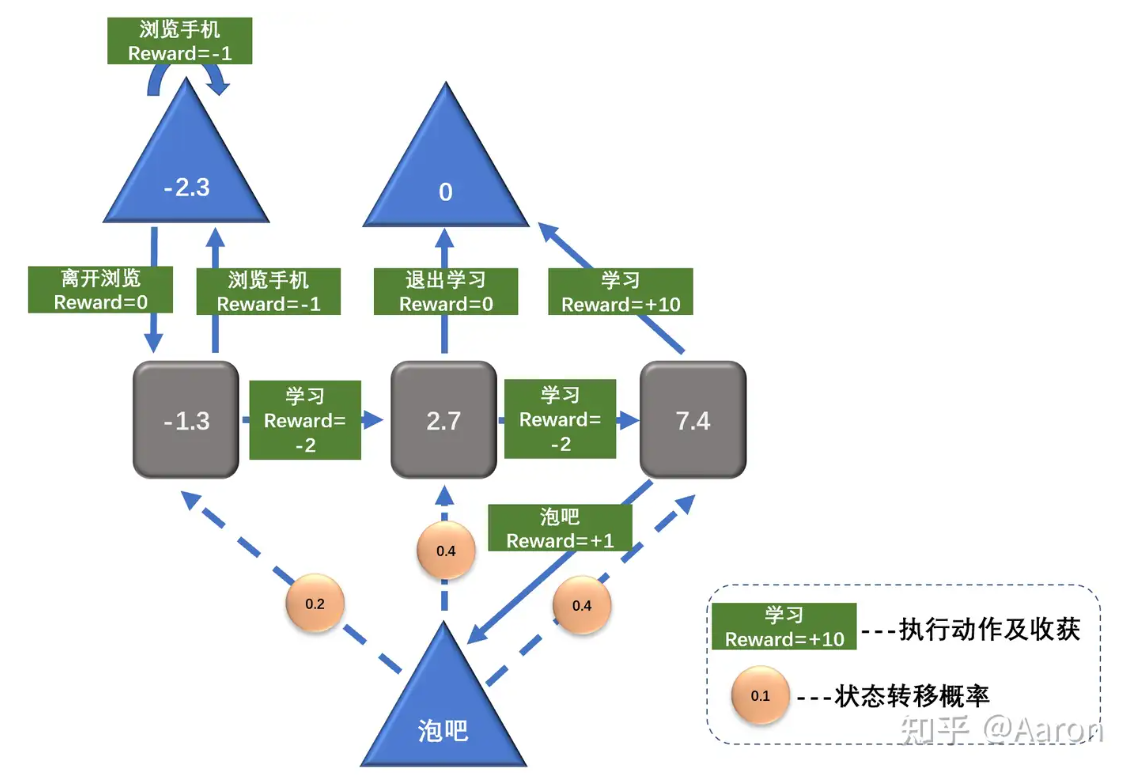
As we can see, the value of each state not only includes its own reward but also the rewards of “all states that can be reached from this state.” The gamma factor determines how much we value future rewards.

Returning to the student example, let’s assume that in the third lecture, the probabilities of hanging out and studying are both 0.5 (a fixed policy) and the decay factor γ is 1. It turns out that although the reward for attending the third lecture seems like -2, its actual value can be as high as 7.4:

Influence

Keywords: Social Network

Some people reach the friend limit on WeChat, while others have only a few friends. A report from a few years ago indicated that 4% of people have over 1000 WeChat friends, while 59% have between 50 and 500 friends. So, does having more WeChat friends equate to greater influence?

In networks, there’s a concept called “centrality,” which measures a node’s importance within a network. Centrality can be calculated in several ways, but the core idea is to look at the node’s connections. In other words, in a social circle, your value is not determined by you but by how those around you perceive you.

The three most common methods for calculating centrality are degree centrality, betweenness centrality, and closeness centrality.

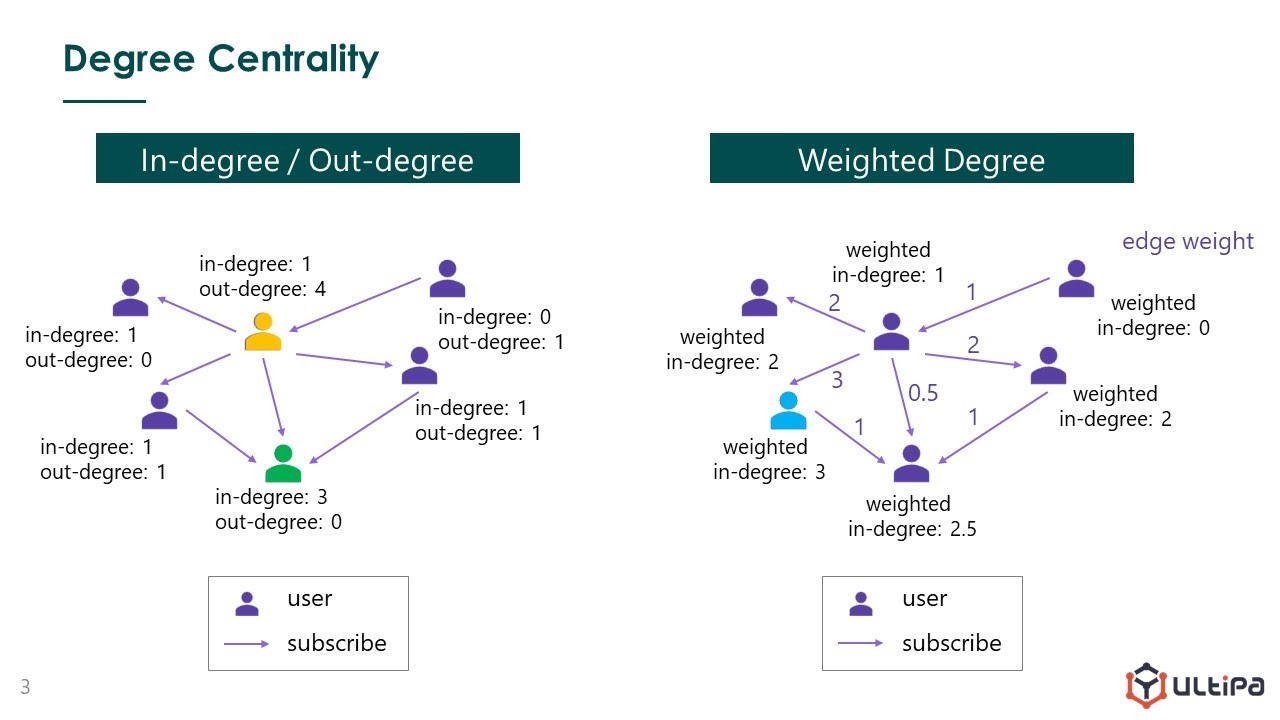
Degree centrality is intuitive—the more connections, the higher the degree centrality:

Betweenness centrality is different. It measures the “key intermediary”:

\[ g(v) = \sum_{s \neq v \neq t} \frac{\sigma_{s t}(v)}{\sigma_{s t}} \]

where \( \sigma_{s t} \) represents the total number of shortest paths between nodes \( s \) and \( t \), and \( \sigma_{s t}(v) \) represents the number of those paths that pass through \( v \).

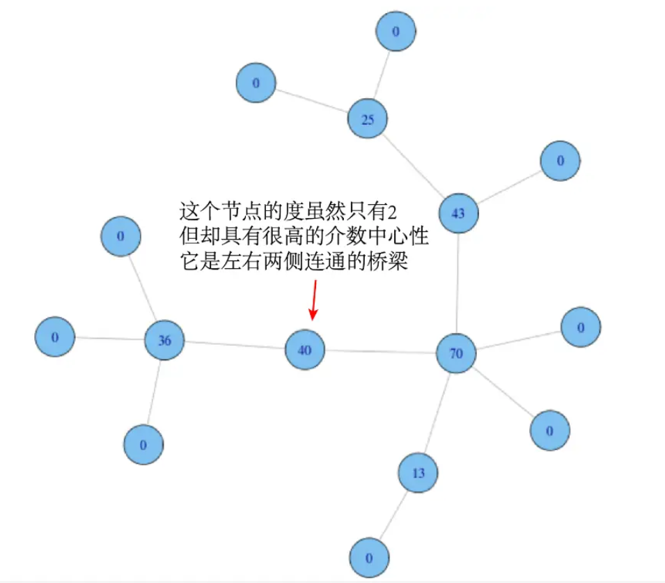
This means that besides the number of links, another dimension for measuring a node’s importance emphasizes a node’s intermediary role within the network. It evaluates whether information or resources among other people in the network must necessarily pass through you.

In social circles, instead of adding thousands of friends, it may be more effective to become a “key person” in an intersectional field, acting as a bridge between two or more domains.

Closeness centrality resembles geometric centrality. It’s calculated based on the shortest path between all node pairs, as well as the sum of distances from each node to all others. This value is then inverted to determine the node’s closeness centrality score:

\[ C(u) = \frac{1}{\sum_{v-1}^{n-1} d(u, v)} \]

This means that if a node has very short shortest-path distances to other nodes, its closeness centrality is high.

In an organization with a flat reporting structure, the boss would have high closeness centrality, as they are near every node. Conversely, adding layers and departments reduces this value—one reason why NVIDIA’s CEO wants to hear as many reports as possible.

As for us, it’s challenging to change an entire network structure to make oneself the geometric center. A more achievable strategy might be to pursue a high betweenness centrality score by becoming a “key intermediary” in overlapping fields.

Path Dependence

Keywords: Stationarity

In a box with black and white balls, the more you draw, the better you can estimate their distribution. This is classical probability from centuries ago.

However, modern mathematics reveals the concept of stationarity. Imagine if, after each draw, a machine in the box produces or destroys black and white balls at random. Regardless of how many draws are taken, you can never estimate the distribution of balls in the box.

This concept tells us not to rely on “path dependence” in life or trust any calm surface. Real life is far trickier than a ball-drawing game—draw 100 times for white balls, and next might be a golden egg or even a python.

Jean-Manuel Rozan, founder of DeepL, once worked as a banker. He wrote: “I often played tennis with George Soros on Long Island and sometimes talked about the financial market. One weekend, Soros expressed his deep bearish view, explaining it with complex reasoning that I couldn’t follow. Soros had clearly shorted the market.”

A few days later, the market surged. Concerned, I asked him if he lost money. “We made a fortune,” he said. “I changed my mind and took a long position.”

True speculators like Soros are unique—they lack path dependence and treat each day as a blank slate. They never assume that the next draw will be a black ball just because the previous one was.

This approach inspired Rozan to shift from finance to AI, founding Qwant and later DeepL.

Many people hold on to their beliefs until they reach the grave.

Asymmetric Opportunities

Keywords: Skewness

There is often debate over bull and bear markets. A bull market is when most stocks likely rise, while a bear market sees most stocks likely fall.

But a bull market doesn’t necessarily mean buying is optimal, because opportunities are often asymmetric.

Consider the Peso Problem, a classic issue in economics. The Argentinian Peso remained stable against the dollar for a long time, but historically experienced occasional sharp devaluations.

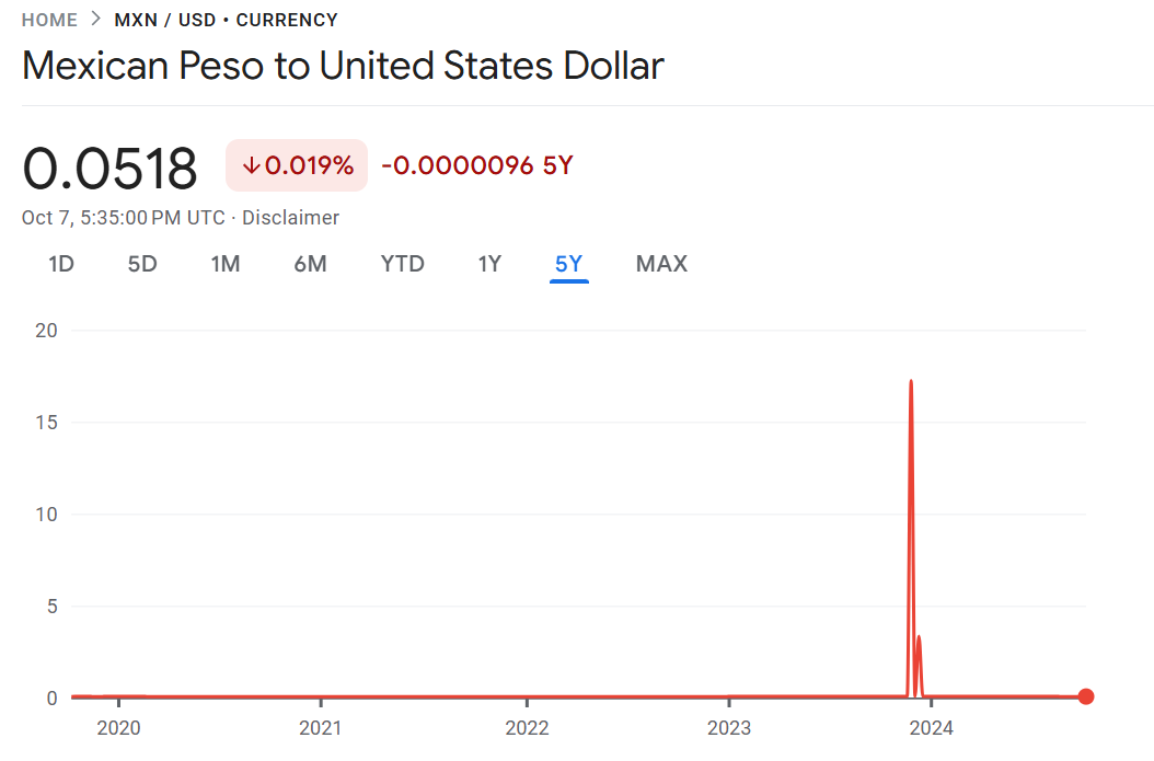
A skilled trader repeatedly trading Pesos might earn steady small gains. But if leverage is high, a sudden fluctuation could be devastating, as stable periods and major swings are asymmetric.

Returning to the bull vs. bear market, a great trader might short a bull market due to these asymmetries. Although the market has a 70% chance of rising by 1%, there’s a 10% chance of a 10% drop. A great trader will profit from betting on rare events, incurring small losses but ultimately winning big.

This asymmetry is why most retail investors lose money in bull markets. Although Bitcoin’s price has surged to $60,000, most speculators lose. They may profit for weeks but eventually capitulate during an unexpected crash.

Another asymmetric opportunity is right before you—adding me on WeChat. You’ll spend only a few minutes, but this small time investment could yield significant returns.