Tensor Parallelism and NCCL

Recommend Reading: https://uvadlc-notebooks.readthedocs.io/en/latest/tutorial_notebooks/scaling/JAX/tensor_parallel_simple.html

1. Transformer Architecture Overview

1. Input Embedding Layer:

   • Converts input tokens (e.g., words) into dense vectors of fixed size.
   • Adds positional encoding to incorporate sequential information.

2. Multi-Head Self-Attention:

   • Captures global dependencies between different positions in the sequence.

3. Feed-Forward Network (FFN):

   • Applies independent transformations to each position in the sequence.

4. Layer Normalization and Residual Connections:

   • Stabilizes training and improves convergence.

5. Output Layer:

   • Maps the processed features into probabilities over the output vocabulary.

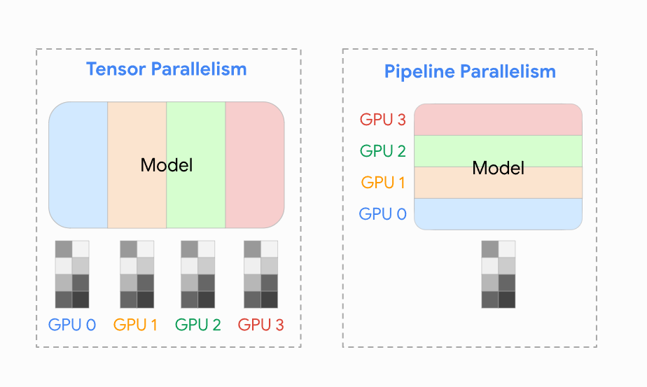
Tensor Parallelism optimizes the computation of large matrix operations in self-attention and FFN layers.

---

2. Tensor Parallelism in Transformers

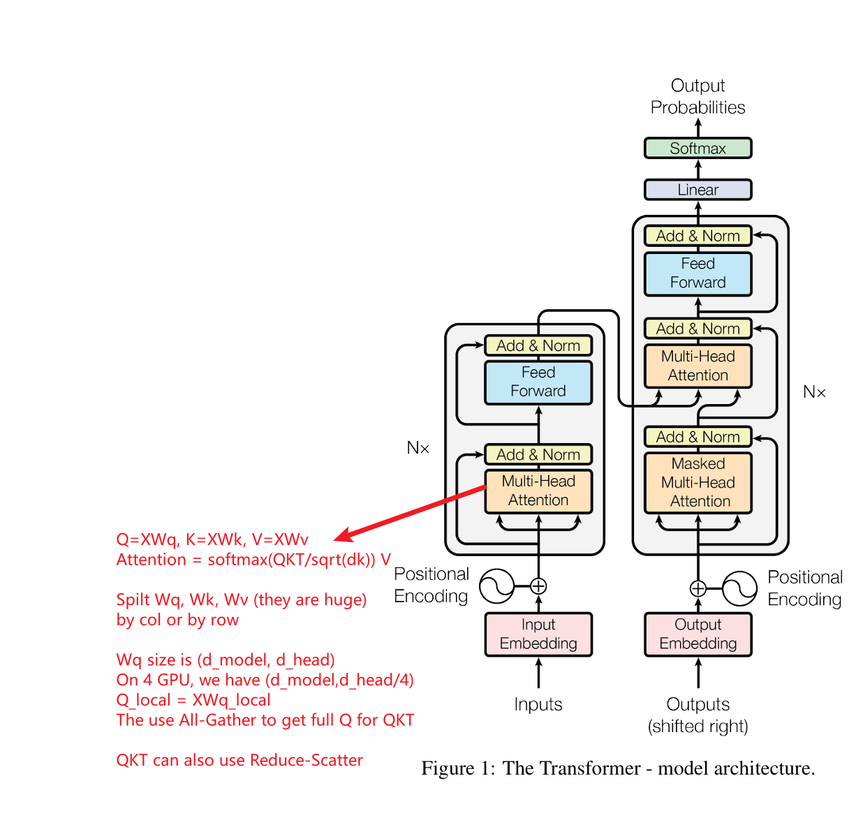
2.1 Multi-Head Self-Attention with Tensor Parallelism

Self-attention operates as follows:

$$\text{Attention}(Q, K, V) = \text{Softmax}\left(\frac{QK^\top}{\sqrt{d_k}}\right)V$$

Where:

• $Q$, $K$, $V$ are derived from the input $X$ via weight matrices $W_Q$, $W_K$, and $W_V$:

$$Q = XW_Q, \quad K = XW_K, \quad V = XW_V$$

Tensor Parallelism Steps:

1. Weight Matrix Partitioning:

   • Split $W_Q$, $W_K$, $W_V$ across GPUs.
   • For example, if $W_Q$ has shape $d_{\text{model}} \times d_{\text{head}}$ and there are 4 GPUs, each GPU stores $d_{\text{model}} \times (d_{\text{head}} / 4)$.

2. Parallel Computation:

   • Each GPU independently computes its portion of $Q$:

     $$Q_{\text{local}} = XW_{Q,\text{local}}$$

3. All-Gather Communication:

   • Combine $Q_{\text{local}}$ from all GPUs into the full $Q$ using All-Gather.

4. Distributed Matrix Multiplication:

   • Partition $Q$ and $K$ for efficient parallel computation of $QK^\top$.
   • Use Reduce-Scatter to aggregate partial results.

5. Weighted Sum with $V$:

   • Each GPU computes its part of $V$ and synchronizes the output using Reduce-Scatter.

---

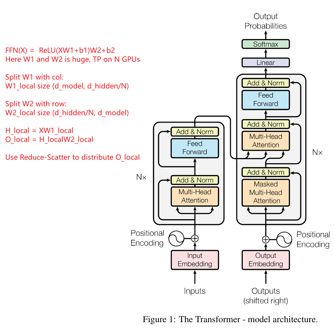
2.2 Feed-Forward Network (FFN) with Tensor Parallelism

The FFN applies two linear transformations with intermediate activation:

$$\text{FFN}(X) = \text{ReLU}(XW_1 + b_1)W_2 + b_2$$

Where:

• $W_1$: $d_{\text{model}} \times d_{\text{hidden}}$
• $W_2$: $d_{\text{hidden}} \times d_{\text{model}}$

Tensor Parallelism Steps:

1. Weight Matrix Partitioning:

   • Split $W_1$ along columns and $W_2$ along rows.
   • Each GPU holds:
     • $W_1$: $d_{\text{model}} \times (d_{\text{hidden}} / N)$
     • $W_2$: $(d_{\text{hidden}} / N) \times d_{\text{model}}$

2. Forward Computation:

   • Each GPU computes: $$H_{\text{local}} = XW_{1,\text{local}}$$

3. Synchronization:

   • Use All-Gather to combine $H_{\text{local}}$ into $H$.

4. Second Linear Transformation:

   • Each GPU computes: $$O_{\text{local}} = HW_{2,\text{local}}$$

5. Result Synchronization:

   • Use Reduce-Scatter to distribute $O_{\text{local}}$ across GPUs.

---

3. Training Process of Tensor Parallel Transformers

3.1 Input Handling

• Tokenized input sequences are embedded and distributed among GPUs.

3.2 Forward Pass

1. Multi-Head Self-Attention:

   • Each GPU computes its part of $Q$, $K$, $V$ using local weights.
   • Synchronize results using All-Gather and compute attention scores in parallel.

2. Feed-Forward Network:

   • Each GPU performs partitioned linear transformations.
   • Use All-Gather and Reduce-Scatter to synchronize intermediate results.

3.3 Loss Computation and Backward Pass

1. Gradient Computation:

   • Each GPU computes local gradients for its partitioned weights.

2. Gradient Synchronization:

   • Use All-Reduce to synchronize gradients across GPUs.

3. Weight Updates:

   • Each GPU updates its local weights using synchronized gradients.

---

NCCL

1. All-Reduce

• Function: Aggregates data from all GPUs (e.g., summation) and broadcasts the result back to all GPUs.
• Topology Used: Ring Topology.
• Communication Process:
  1. Each GPU sends its data to the next GPU while receiving data from the previous GPU.
  2. Each communication round performs part of the Reduce operation.
  3. During the broadcast phase, the final result is synchronized across all GPUs.

ASCII Diagram

Step 1: Reduce Phase (Ring Summation)
  GPU0 -> GPU1 -> GPU2 -> GPU3
  Data flows in the ring and accumulates:
    GPU0: [1, 2] + GPU1: [3, 4]
    GPU1: [4, 6] -> GPU2: [9, 10] + ...

Step 2: Broadcast Phase (Ring Broadcast)
  GPU3 -> GPU2 -> GPU1 -> GPU0
  Each GPU receives the final result: [16, 20]

Ring Topology:
  GPU0 → GPU1 → GPU2 → GPU3
    ↑                     ↓
    ←---------------------←

---

2. Reduce

• Function: Aggregates data from all GPUs, with the result stored on a specified Root GPU.
• Topology Used: Tree Topology.
• Communication Process:
  1. Data is progressively aggregated to the Root GPU following a tree structure.
  2. Each GPU passes its data to its parent and performs the Reduce operation.

ASCII Diagram

Tree Topology:
       GPU0 (Root)
       /    \
    GPU1    GPU2
    /          \
 GPU3         GPU4

Step 1: Each pair of GPUs merges data
  GPU3 + GPU1 → GPU1: [A+B]
  GPU4 + GPU2 → GPU2: [C+D]

Step 2: Upper levels continue merging
  GPU1 + GPU2 → GPU0: [SUM(A, B, C, D)]

---

3. Broadcast

• Function: Broadcasts data from the Root GPU to all other GPUs.
• Topology Used: Tree Topology.
• Communication Process:
  1. The Root GPU transmits data to the next level of GPUs.
  2. Each GPU forwards the received data to its children until all GPUs are synchronized.

ASCII Diagram

Tree Topology:
       GPU0 (Root)
       /    \
    GPU1    GPU2
    /          \
 GPU3         GPU4

Step 1: Root broadcasts to child nodes
  GPU0 -> GPU1, GPU2: Data synchronized
Step 2: Child nodes broadcast further
  GPU1 -> GPU3, GPU2 -> GPU4

---

4. All-Gather

• Function: Each GPU gathers data from all other GPUs, resulting in each GPU having complete data.
• Topology Used: Ring Topology.
• Communication Process:
  1. Each GPU sends its data block to the next GPU and receives data from the previous GPU.
  2. After ( N-1 ) communication rounds, all GPUs have collected the complete data.

ASCII Diagram

Ring Topology:
  GPU0 → GPU1 → GPU2 → GPU3
    ↑                     ↓
    ←---------------------←

Step 1: Each GPU sends its data
  GPU0 sends [A] to GPU1, GPU1 sends [B] to GPU2...

Step 2: Data rotates and accumulates
  Each GPU collects one new block per round until all blocks are gathered:
  GPU0 -> [A, B, C, D]
  GPU1 -> [A, B, C, D]
  ...

---

5. Reduce-Scatter

• Function: Aggregates data across all GPUs in chunks (Reduce) and distributes the aggregated chunks to all GPUs (Scatter).
• Topology Used: Ring Topology.
• Communication Process:
  1. Each GPU sends and receives data in chunks, performing the Reduce operation on the received data.
  2. Eventually, each GPU has a chunk of the globally aggregated result.

ASCII Diagram

Step 1: Data is divided into chunks
  GPU0: [A0, A1], GPU1: [B0, B1], ...
Step 2: Ring Reduce
  GPU0 sends A1 to GPU1, GPU1 sends B1 to GPU2...
  Aggregated results are distributed in chunks:
  GPU0: [A0+B0+C0+D0]
  GPU1: [A1+B1+C1+D1]

Ring Topology:
  GPU0 → GPU1 → GPU2 → GPU3
    ↑                     ↓
    ←---------------------←

---

6. Scatter

• Function: Splits the data on the Root GPU into chunks and distributes them to all GPUs.
• Topology Used: Tree Topology.
• Communication Process:
  1. The Root GPU splits the data into chunks.
  2. Each chunk is transmitted to the corresponding GPU following a tree structure.

ASCII Diagram

Tree Topology:
       GPU0 (Root)
       /    \
    GPU1    GPU2
    /          \
 GPU3         GPU4

Step 1: Root splits and distributes data
  GPU0 sends [A] to GPU1, [B] to GPU2
Step 2: Child nodes distribute further
  GPU1 sends [C] to GPU3, GPU2 sends [D] to GPU4

---

7. Gather

• Function: Collects data from all GPUs and consolidates it on the Root GPU.
• Topology Used: Tree Topology.
• Communication Process:
  1. Each GPU sends its data to its parent node.
  2. Data is progressively aggregated and consolidated at the Root GPU.

ASCII Diagram

Tree Topology:
       GPU0 (Root)
       /    \
    GPU1    GPU2
    /          \
 GPU3         GPU4

Step 1: Child nodes send data upwards
  GPU3 sends [A] to GPU1, GPU4 sends [B] to GPU2
Step 2: Parent nodes merge data
  GPU1 + GPU2 -> GPU0

---

Summary

Communication Strategy	Topology	Features
All-Reduce	Ring Topology	Global aggregation and broadcast using ring Reduce + Broadcast
Reduce	Tree Topology	Global aggregation to Root GPU
Broadcast	Tree Topology	Data broadcasted from Root to all devices
All-Gather	Ring Topology	All data gathered to each GPU
Reduce-Scatter	Ring Topology	Partial aggregation and scatter
Scatter	Tree Topology	Root data split and distributed
Gather	Tree Topology	Data consolidated at Root GPU

The choice of strategy depends on the application scenario and data characteristics. Feel free to ask for more details about any specific operation!

Step by Step Example of NCCL

Understanding Reduce-Scatter: A Step-by-Step Guide

The Reduce-Scatter operation combines two main steps:

1. Reduce: Perform a specified operation (e.g., SUM) on corresponding blocks of data across GPUs.
2. Scatter: Distribute the reduced results to specific GPUs.

The key idea is to efficiently distribute the computation and communication workload, ensuring each GPU holds a unique portion of the reduced global data.

---

SUM Operation Rule

In Reduce-Scatter, the SUM operation applies to corresponding chunks of data across GPUs. It’s important to note:

• The SUM operation is not applied to the entire tensor globally.
• Instead, the tensor is divided into chunks, and the SUM is performed locally on each chunk (Reduce). The resulting reduced chunks are then distributed (Scatter) to the GPUs.

As a result, each GPU contains only a part of the global reduced data, not the sum of the entire tensor.

---

Example Analysis

Let’s clarify with an example of 4 GPUs, where each GPU starts with a tensor of values:

• GPU0: ([1, 2, 3, 4])
• GPU1: ([5, 6, 7, 8])
• GPU2: ([9, 10, 11, 12])
• GPU3: ([13, 14, 15, 16])

Step 1: Divide the Data into Chunks

Each tensor is evenly divided into 4 chunks, one for each position:

• GPU0: ([1], [2], [3], [4])
• GPU1: ([5], [6], [7], [8])
• GPU2: ([9], [10], [11], [12])
• GPU3: ([13], [14], [15], [16])

Step 2: Perform the Reduce Operation (SUM)

For each position (i), perform the SUM operation across all GPUs:

• Chunk 0 (position 0 across all GPUs):

  $$R_0 = 1 + 5 + 9 + 13 = 28$$

• Chunk 1 (position 1 across all GPUs):

  $$R_1 = 2 + 6 + 10 + 14 = 32$$

• Chunk 2 (position 2 across all GPUs):

  $$R_2 = 3 + 7 + 11 + 15 = 36$$

• Chunk 3 (position 3 across all GPUs):

  $$R_3 = 4 + 8 + 12 + 16 = 40$$

Step 3: Scatter the Results

Distribute the reduced chunks to the GPUs:

• GPU0 receives (R_0 = 28).
• GPU1 receives (R_1 = 32).
• GPU2 receives (R_2 = 36).
• GPU3 receives (R_3 = 40).

---

Why Are Results Different on Each GPU?

In Reduce-Scatter, the goal is not for each GPU to hold the result of the global tensor reduction. Instead, each GPU retains only the reduced result of the chunk it is responsible for. This design ensures:

• Each GPU processes a smaller portion of the data.
• Communication overhead is reduced, as GPUs share only the chunks relevant to their tasks.

---

Applications and Advantages

1. Reducing Communication Overhead:

   • In operations like All-Reduce, all GPUs would hold the entire reduced tensor, leading to higher communication costs.
   • Reduce-Scatter minimizes communication by only transferring reduced chunks.

2. Distributed Training:

   • During training, GPUs often require only specific portions of gradients or parameters.
   • Reduce-Scatter ensures that each GPU gets only the data it needs, making training more efficient.

---

Summary: Rules and Concepts

1. Reduce Rule:

   • Divide the tensor into chunks and perform the operation (e.g., SUM) across corresponding chunks on all GPUs.
   • For SUM, each reduced chunk is: $$R_i = A_{0,i} + A_{1,i} + \cdots + A_{N-1,i}$$

2. Scatter Rule:

   • Distribute each reduced chunk (R_i) to its corresponding GPU.

3. Why GPUs Hold Different Results:

   • Each GPU retains only one part of the global reduced data. This reduces memory and communication costs.

4. Advantages:

   • Efficiency: Less communication and memory usage.
   • Scalability: Ideal for large-scale distributed systems.